How to do a Kaggle Competition AND do it right!
by CM
Posted on December 31, 2019

The Goal:
As already mentioned in the first article, Kaggle is an online community of data scientists and machine learners that allows users to find and publish data sets, explore and build models in a web-based data-science environment, and enter competitions to tackle data science challenges. In outcome, Kaggle provides ML competitions, public data sets, a cloud-based workbench for data science, and short form AI education. In this article, we explore Kaggle to participate in a Kaggle competition. In this regard, we will enter the Kannada MNIST competition. This competition holds an MNIST like datatset for Kannada handwritten digits. In other words, the goal of this competition is to provide an extension to the classic MNIST competition we're all familiar with. Instead of using Arabic numerals, it uses a recently-released dataset of Kannada digits.
Key components are:
Dataset:
- Kaggle Source (.csv Format)
Note: That this article uses a Convolutional Neural Network (CNN, or ConvNet) to tackle the Kaggle competion. Hence, we will explore a class of deep neural networks, that is commonly applied to analyzing visual imagery. First, we will go on Kaggle on look for competitions. In the search field, enter: "Kannada MNIST". You will be directed to the Playground Code Competition -- Kannada MNIST.

On the landing page, we need to have a look at five things:
- (1) Description
- (2) Evaluation
- (3) The Timeline
- (4) Kernel Requirements
- (5) Data

(1) In the DESCRIPTION, we usually get the infomration what the challenge is about, respectively what we will later predict using the provided data. In other words, the tasks including useful background information can be found in this section. (2) EVALUATION gives us the information how the competition is evaluated, e.g. accuracy of our predictions (the percentage of images we get correct). Further, we find the exact format the our final "Submission file" needs to have in order to get accepted to enter the competition. As the name suggest, (3) TIMELINE a) Entry deadline, (b) Team Merger deadline, and (c) Final Submission Deadline. (4) KERNEL REQUIREMENTS gives us insights on the platform to run our Jupyter notebooks in the browser.
Under (5) Data, we usually find the training and test data that we can use for building our model.

In the given competition, we will try to correctly classify images to respective numbers (0-9). So let's get to the basics first. I already mentioned that we will use a CNN in our model. CNN is powerful and widely used across image and video recognition, recommender systems, image classification, medical image analysis, and natural language processing. A "Convolutional Neural Network" generally defines that the network employs a mathematical function called convolution. This convolution is a kind of matrix multiplication of an input and a kernel. In our example, the input refers to an 'image' and respective pixel values and the kernel to a pre-defined filter. The multiplication leads to an output which will be added up to a single value. The picture below shows an example of such a convolutional operation:

But why do we use convolutional operations in the first place? The answer goes down to the fact that we want to detect e.g. patterns such as shapes or lines in our pictures that leads us to the final decision on making the correct prediction. Hence, in order to allow for this 'pattern recognition', we leverage filters. Each filter has the job of detecting a different shape or pattern in our image, although the task of the filter becomes increasingly complex in the deeper layers of our network. In summary, we use filters to extract 'patterns' in our image. After the extraction, we generally employ a fully connected layer for classification.
What is Padding and why is it useful?
Padding refers to the process of symmetrically adding values to the input matrix. In other words, padding is simply a process of adding layers of zeros to our input images to avoid edge, and corner pixel problems.

The pixels at the edges of an images are convoluted only once, while the pixels in the middle are convoluted 5 times with a 5x5 filter. This results in the loss of pixel information on the edges. The idea of adding a padding is that edge pixels can be convoluted multiple times as well. Another advantage of padding is to preserve the output dimensions as convolution operation generally lead to a reduction of the output matrix.
What is Pooling and why is it useful?
Convolutional networks often include local or global pooling layers to streamline the underlying computation. Pooling layers reduce the dimensions of the input by combining the outputs of neuron clusters at one layer into a single neuron in the next layer. For example, Max pooling uses the maximum value from each of a cluster of neurons at the prior layer, On the other hand, Average pooling uses the average value from each of a cluster of neurons at the prior layer. In summary, Pooling layers downsample sample features.

Pooling is useful to increase robustness on feature extraction, as pooling prevents the model from over-training by discarding the unnecessary data relative to the selected value. Furthermore, Pooling allows to speed up the computation by reducing the size of the representation.
What is Batch Normalization and why is it useful?
Batch Normalization is a technique used to normalize the input layer by adjusting and scaling the activations. Batch normalization further is used for improving speed, performance, and stability of a neural network. In other words, Batch Normalization is technique that converts the outputs of a neural network into a standard format. This effectively 'resets' the output of the previous layer that it can be efficiently processed by the follwoing layer.

What is Dropout and why is it useful?
Drop out is a regularization method. In training, some nodes are randomly ignored or "dropped out." This has the effect of making the layer look-like and be treated-like a layer with a different number of nodes and connectivity to the prior layer. This helps to avoid overfitting and allows better generalization in deep neural networks of all kinds. Hence, Dropout offers a very computationally cheap and remarkably effective regularization method that can be employed with most types of layers, such as dense fully connected layers, convolutional layers, and recurrent layers.
After we got the theory in, we will start coding. First, we import all our dependencies:
import pandas as pd
import numpy as np
import matplotlib.pyplot as plt

import tensorflow as tf
from tensorflow.keras.models import Sequential
from tensorflow.keras.layers import Conv2D, MaxPooling2D, Flatten, Dropout, Dense, BatchNormalization, LeakyReLU
from tensorflow.keras.preprocessing.image import ImageDataGenerator
from tensorflow.keras.callbacks import ReduceLROnPlateau, EarlyStoppingntial
from tensorflow.keras.layers import Dense
Second, we load the training and test data into pandas dataframes using the pd.rad_csv function. In this regard, we need to have a look in what file-format the training and test data is -- in our competition the data is available as CSV files. We find the data and the respective path under "input/Kannada MNIST"
training = pd.read_csv("../input/Kannada-MNIST/train.csv")
test = pd.read_csv("../input/Kannada-MNIST/test.csv")
print(test.head())
When printing test.head(), we find the first five rows of the our test data. As mentioned on the data tab, we find that we have 784 columns of pixel data and one "id column".
==========================
OUTPUT
==========================

id  pixel0  pixel1  pixel2  pixel3  pixel4  pixel5  pixel6  pixel7  pixel8  \
0   0       0       0       0       0       0       0       0       0       0
1   1       0       0       0       0       0       0       0       0       0
2   2       0       0       0       0       0       0       0       0       0
3   3       0       0       0       0       0       0       0       0       0
4   4       0       0       0       0       0       0       0       0       0

...  pixel774  pixel775  pixel776  pixel777  pixel778  pixel779  pixel780  \
0  ...         0         0         0         0         0         0         0
1  ...         0         0         0         0         0         0         0
2  ...         0         0         0         0         0         0         0
3  ...         0         0         0         0         0         0         0
4  ...         0         0         0         0         0         0         0

pixel781  pixel782  pixel783
0         0         0         0
1         0         0         0
2         0         0         0
3         0         0         0
4         0         0         0

[5 rows x 785 columns]
With respect to data processing, we need to transform the dataframe into numpy arrays. We do this, as we then can easiliy slice the array in the wanted structure: depedent variable (y value) and our input features (x values). Using the newly build arrays, we can easily apply a tensor tranformation and use them in our keras model later on.
#Dataframe to Array
  training_array = np.array(training)

#Slicing arrays
x_train = training_array[:,1:]
y_train = training_array[:,0]

#Transforming to tensor
x_train = tf.constant(x_train)
y_train = tf.constant(y_train)

#Normalizing pixel value betweenn 0-1
x_train = tf.keras.utils.normalize(x_train, axis=1)

#We repeat these steps for the test data as well
test_array = np.array(test)
x_test = test_array[:,1:]
y_test = test_array[:,0]

x_test = tf.constant(x_test)
x_test = tf.keras.utils.normalize(x_test, axis=1)
y_test = tf.constant(y_test)
Next step is to reshape the arrays that they will represent a 28x28 image.
x_train = x_train.reshape(x_train.shape[0], 28, 28, 1)
x_test =  x_test.reshape(x_test.shape[0], 28, 28, 1)

x_train = tf.constant(x_train)
x_test = tf.constant(x_test)
We now employ the Keras function ImageDataGenerator, which rotates and shifts our images which later helps the model to generalize better. In other words, ImageDataGenerator does not generate new Images but changes the appearance of the images using transformation.
datagen_train = ImageDataGenerator(rotation_range = 10,
                                   width_shift_range = 0.25,
                                   height_shift_range = 0.25,
                                   shear_range = 0.1,
                                   zoom_range = 0.35,
                                   horizontal_flip = False)

datagen_val = ImageDataGenerator()
We then start building the model (Sequential). We use a combination of convolutional and dense layers, while applying normalization, pooling, activation, and dropouts after the respective layers.
model = Sequential()
model.add(Conv2D(filters =64, kernel_size=(3,3), padding='same', input_shape = [28,28,1]))
model.add(BatchNormalization(momentum=0.9, epsilon=1e-5, gamma_initializer="uniform"))
model.add(LeakyReLU(alpha=0.1))
model.add(Conv2D(filters =64, kernel_size=(3,3), padding='same'))
model.add(BatchNormalization(momentum=0.9, epsilon=1e-5, gamma_initializer="uniform"))
model.add(LeakyReLU(alpha=0.1))
model.add(Conv2D(filters =64, kernel_size=(3,3), padding='same'))
model.add(BatchNormalization(momentum=0.9, epsilon=1e-5, gamma_initializer="uniform"))
model.add(LeakyReLU(alpha=0.1))
model.add(MaxPooling2D(2, 2))
model.add(Dropout(0.25))

model.add(Conv2D(filters =128, kernel_size=(3,3), padding='same', input_shape = [28,28,1]))
model.add(BatchNormalization(momentum=0.9, epsilon=1e-5, gamma_initializer="uniform"))
model.add(LeakyReLU(alpha=0.1))
model.add(Conv2D(filters =128, kernel_size=(3,3), padding='same'))
model.add(BatchNormalization(momentum=0.9, epsilon=1e-5, gamma_initializer="uniform"))
model.add(LeakyReLU(alpha=0.1))
model.add(Conv2D(filters =128, kernel_size=(3,3), padding='same'))
model.add(BatchNormalization(momentum=0.9, epsilon=1e-5, gamma_initializer="uniform"))
model.add(LeakyReLU(alpha=0.1))
model.add(MaxPooling2D(2, 2))
model.add(Dropout(0.25))

model.add(Conv2D(filters =256, kernel_size=(3,3), padding='same', input_shape = [28,28,1]))
model.add(BatchNormalization(momentum=0.9, epsilon=1e-5, gamma_initializer="uniform"))
model.add(LeakyReLU(alpha=0.1))
model.add(Conv2D(filters =256, kernel_size=(3,3), padding='same'))
model.add(BatchNormalization(momentum=0.9, epsilon=1e-5, gamma_initializer="uniform"))
model.add(LeakyReLU(alpha=0.1))
model.add(Conv2D(filters =256, kernel_size=(3,3), padding='same'))
model.add(BatchNormalization(momentum=0.9, epsilon=1e-5, gamma_initializer="uniform"))
model.add(LeakyReLU(alpha=0.1))
model.add(MaxPooling2D(2, 2))
model.add(Dropout(0.25))

model.add(Flatten())

model.add(Dense(units = 80, input_shape = (784,), activation='relu'))
model.add(Dense(units = 120, input_shape = (80,), activation='relu'))
model.add(Dense(units = 10, input_shape = (120,), activation='softmax'))
We can have a look at our model summary.
==========================
OUTPUT
==========================

Model: "sequential"
_________________________________________________________________
Layer (type)                 Output Shape              Param #
=================================================================
conv2d (Conv2D)              (None, 28, 28, 64)        640
_________________________________________________________________
batch_normalization (BatchNo (None, 28, 28, 64)        256
_________________________________________________________________
leaky_re_lu (LeakyReLU)      (None, 28, 28, 64)        0
_________________________________________________________________
conv2d_1 (Conv2D)            (None, 28, 28, 64)        36928
_________________________________________________________________
batch_normalization_1 (Batch (None, 28, 28, 64)        256
_________________________________________________________________
leaky_re_lu_1 (LeakyReLU)    (None, 28, 28, 64)        0
_________________________________________________________________
conv2d_2 (Conv2D)            (None, 28, 28, 64)        36928
_________________________________________________________________
batch_normalization_2 (Batch (None, 28, 28, 64)        256
_________________________________________________________________
leaky_re_lu_2 (LeakyReLU)    (None, 28, 28, 64)        0
_________________________________________________________________
max_pooling2d (MaxPooling2D) (None, 14, 14, 64)        0
_________________________________________________________________
dropout (Dropout)            (None, 14, 14, 64)        0
_________________________________________________________________
conv2d_3 (Conv2D)            (None, 14, 14, 128)       73856
_________________________________________________________________
batch_normalization_3 (Batch (None, 14, 14, 128)       512
_________________________________________________________________
leaky_re_lu_3 (LeakyReLU)    (None, 14, 14, 128)       0
_________________________________________________________________
conv2d_4 (Conv2D)            (None, 14, 14, 128)       147584
_________________________________________________________________
batch_normalization_4 (Batch (None, 14, 14, 128)       512
_________________________________________________________________
leaky_re_lu_4 (LeakyReLU)    (None, 14, 14, 128)       0
_________________________________________________________________
conv2d_5 (Conv2D)            (None, 14, 14, 128)       147584
_________________________________________________________________
batch_normalization_5 (Batch (None, 14, 14, 128)       512
_________________________________________________________________
leaky_re_lu_5 (LeakyReLU)    (None, 14, 14, 128)       0
_________________________________________________________________
max_pooling2d_1 (MaxPooling2 (None, 7, 7, 128)         0
_________________________________________________________________
dropout_1 (Dropout)          (None, 7, 7, 128)         0
_________________________________________________________________
conv2d_6 (Conv2D)            (None, 7, 7, 256)         295168
_________________________________________________________________
batch_normalization_6 (Batch (None, 7, 7, 256)         1024
_________________________________________________________________
leaky_re_lu_6 (LeakyReLU)    (None, 7, 7, 256)         0
_________________________________________________________________
conv2d_7 (Conv2D)            (None, 7, 7, 256)         590080
_________________________________________________________________
batch_normalization_7 (Batch (None, 7, 7, 256)         1024
_________________________________________________________________
leaky_re_lu_7 (LeakyReLU)    (None, 7, 7, 256)         0
_________________________________________________________________
conv2d_8 (Conv2D)            (None, 7, 7, 256)         590080
_________________________________________________________________
batch_normalization_8 (Batch (None, 7, 7, 256)         1024
_________________________________________________________________
leaky_re_lu_8 (LeakyReLU)    (None, 7, 7, 256)         0
_________________________________________________________________
max_pooling2d_2 (MaxPooling2 (None, 3, 3, 256)         0
_________________________________________________________________
dropout_2 (Dropout)          (None, 3, 3, 256)         0
_________________________________________________________________
flatten (Flatten)            (None, 2304)              0
_________________________________________________________________
dense (Dense)                (None, 80)                184400
_________________________________________________________________
dense_1 (Dense)              (None, 120)               9720
_________________________________________________________________
batch_normalization_9 (Batch (None, 120)               480
_________________________________________________________________
dense_2 (Dense)              (None, 10)                1210
=================================================================
Total params: 2,120,034
Trainable params: 2,117,106
Non-trainable params: 2,928
_________________________________________________________________
We can then complile our model. This might take some time due to the complexity and size of the model.
model.compile(loss = 'sparse_categorical_crossentropy', optimizer ='Adam', metrics=['acc'])

history = model.fit(x_train, y_train, verbose=1, epochs=15, batch_size = 100, validation_split = 0.2)
In the training histroy we can see how our model is improving.
Train on 48000 samples, validate on 12000 samples
Epoch 1/15
48000/48000 [==============================] - 926s 19ms/sample - loss: 0.3728 - acc: 0.9729 - val_loss: 0.0486 - val_acc: 0.9870
Epoch 2/15
48000/48000 [==============================] - 908s 19ms/sample - loss: 0.0283 - acc: 0.9928 - val_loss: 0.0267 - val_acc: 0.9927
Epoch 3/15
48000/48000 [==============================] - 916s 19ms/sample - loss: 0.0207 - acc: 0.9941 - val_loss: 0.0213 - val_acc: 0.9939
Epoch 4/15
48000/48000 [==============================] - 913s 19ms/sample - loss: 0.0169 - acc: 0.9950 - val_loss: 0.0149 - val_acc: 0.9958
Epoch 5/15
48000/48000 [==============================] - 913s 19ms/sample - loss: 0.0148 - acc: 0.9956 - val_loss: 0.0176 - val_acc: 0.9958
Epoch 6/15
48000/48000 [==============================] - 911s 19ms/sample - loss: 0.0127 - acc: 0.9962 - val_loss: 0.0192 - val_acc: 0.9946
Epoch 7/15
48000/48000 [==============================] - 915s 19ms/sample - loss: 0.0116 - acc: 0.9965 - val_loss: 0.0219 - val_acc: 0.9942
Epoch 8/15
48000/48000 [==============================] - 912s 19ms/sample - loss: 0.0110 - acc: 0.9966 - val_loss: 0.0255 - val_acc: 0.9933
Epoch 9/15
48000/48000 [==============================] - 920s 19ms/sample - loss: 0.0103 - acc: 0.9966 - val_loss: 0.0175 - val_acc: 0.9948
Epoch 10/15
48000/48000 [==============================] - 912s 19ms/sample - loss: 0.0090 - acc: 0.9973 - val_loss: 0.0194 - val_acc: 0.9954
Epoch 11/15
48000/48000 [==============================] - 911s 19ms/sample - loss: 0.0085 - acc: 0.9974 - val_loss: 0.0296 - val_acc: 0.9934
Epoch 12/15
48000/48000 [==============================] - 911s 19ms/sample - loss: 0.0074 - acc: 0.9977 - val_loss: 0.0410 - val_acc: 0.9899
Epoch 13/15
48000/48000 [==============================] - 910s 19ms/sample - loss: 0.0064 - acc: 0.9981 - val_loss: 0.0223 - val_acc: 0.9952
Epoch 14/15
48000/48000 [==============================] - 912s 19ms/sample - loss: 0.0070 - acc: 0.9979 - val_loss: 0.0140 - val_acc: 0.9966
Epoch 15/15
48000/48000 [==============================] - 910s 19ms/sample - loss: 0.0066 - acc: 0.9977 - val_loss: 0.0323 - val_acc: 0.9908
We find that our model has a great accuracy of 0.9977 (validation accuarcy = 0.9908). In comparison to our fist model (without convolutional layers), we perform much better. Key learning is that the model always need to be adust on the task and data that is porvided upfront.
For the respective competition, we need to have our submission file in a specific format. Our first column should be called 'id', wheras our prediction column should be called 'label'. Hence, in the last step, we both rename the respective columns and make the prediction over the testing data which we will late submit to the competiton.
test_pred = pd.DataFrame(model.predict(x_test))
test_pred = pd.DataFrame(test_pred.idxmax(axis = 1))
test_pred.index.name = 'id'
test_pred = test_pred.rename(columns = {0: 'label'}).reset_index()

sub = test_pred

print(sub.head())
We then transform the newly generated list into numpy arrays.
==========================
OUTPUT
==========================

id  label
0   0      3
1   1      0
2   2      2
3   3      7
4   4      7
In the very last step, we push our submission to the output path in Kaggle.
sub.to_csv('submission.csv',index=False)
After having done this, we can commit our notebook via the commit button -- DONE!.

Commiting might take a couple of minutes.
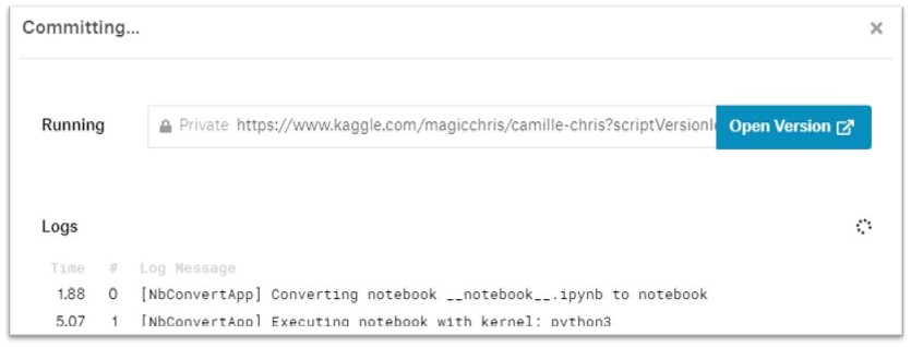
When its finished commiting, we can immediately see our standing on the leaderboard.

We have done it again. We have built a powerful convolutional ML model that allows us to predict the numbers of a 28x28 image. Now it's time to check out the leaderboard ;)